The recent, massive acceleration in ecommerce has created a corresponding increase in online payments fraud. Worldwide, fraud costs businesses more than an estimated $20 billion annually. Plus, for every dollar lost to fraud, the total cost to businesses is actually much higher due to increased operational costs, network fees, and customer churn.
Not only is fraud expensive, but sophisticated fraudsters are constantly finding new ways to exploit weaknesses, making fraud challenging to combat. That’s why we built Stripe Radar, a machine learning–based fraud prevention solution, fully integrated within the Stripe platform. Radar’s machine learning leverages the data from hundreds of billions of dollars in payments processed across the Stripe network each year to accurately detect fraud and quickly adapt to the latest trends, enabling you to grow without increasing fraud.
This guide introduces Stripe Radar and how we leverage the Stripe network to detect fraud, provides an overview of the machine learning techniques we use, explains how we think about the efficacy and performance of fraud detection systems, and describes how other tools in the Radar suite can help businesses optimize their fraud performance.
Introduction to online credit card fraud
A payment is considered fraudulent when the cardholder does not authorize the charge. For example, if a fraudster makes a purchase using a stolen card number that hasn’t been reported, it’s possible the payment would be processed successfully. Then, when the cardholder discovers the fraudulent use of the card, he or she would question the payment with his or her bank by filing a dispute (also known as a “chargeback”).
Businesses can challenge a chargeback by submitting evidence that shows the payment was valid. However, for card-not-present transactions, if the payment is deemed by networks to have been truly fraudulent, the cardholder will win and the business will be liable for the loss of goods and other fees.
Historically, businesses have used brute-force rules to predict and block suspected fraudulent charges. However, hard-coded rules—for example, blocking all credit cards used abroad—may result in blocking many good transactions. Machine learning, on the other hand, can detect more nuanced patterns to help you maximize revenue. In machine learning parlance, a false negative is when the system misses something it is designed to detect—in this case, a fraudulent transaction. A false positive is when the system flags something it shouldn’t have—for example, blocking a legitimate customer. Before we get into the details of machine learning, it’s important to understand the tradeoffs involved.
With false negatives, businesses are often responsible for the original transaction amount plus chargeback fees (the cost associated with the bank reversing the card payment), higher network fees as a result of the dispute, and higher operational costs from reviewing charges or fighting disputes. Plus, if you incur too many disputes, you could end up in a network chargeback monitoring program, which can lead to higher costs or, in some cases, the inability to accept card payments.
False positives, or false declines, are when a legitimate customer tries to make a purchase but is prevented from doing so. False declines can cause the business to take both a gross profit and reputational hit. In fact, in a recent survey, 33% of consumers said they wouldn’t shop again at a business after a false decline.
There is a tradeoff between preventing more disputes (false negatives) and reducing blocking legitimate customers (false positives)—the fewer you have of the former, the more you need to tolerate of the latter (and vice versa). When you prevent more fraud, you’ll increase the number of good customers blocked. On the other hand, reducing the number of false positives often increases the likelihood of more true fraud slipping through the cracks. Businesses need to decide how to balance the two based on their margins, growth profile, and other factors.
If a business’s margins are small (for example, if you sell food online), the cost of a fraudulent transaction might need to be offset with hundreds of good transactions—making each false negative very expensive. Businesses with this profile may lean toward casting a wide net when attempting to stop potential fraud. On the other hand, if a business’s margins are high, say for a SaaS business, the reverse is true. The lost revenue from one legitimate blocked customer may outweigh the cost of increased fraud.
Stripe Radar and the Stripe network
Radar is Stripe’s fraud prevention solution that protects businesses against online credit card fraud. It is powered by adaptive machine learning, the result of years of data science and infrastructure work by Stripe’s dedicated machine learning teams. Radar’s algorithms evaluate every transaction for fraud risk and take action appropriately. High-scoring payments are blocked, and Radar for Fraud Teams provides tools so users can specify when other actions should be taken.
Stripe processes hundreds of billions in payments from millions of businesses and interacts with thousands of partner banks across the globe each year. This scale means we often can see signals and patterns much earlier than smaller networks. Aggregate data relevant to fraud from all Stripe transactions—collected automatically through the payments flow—is used to improve our fraud detection ability. Signals like the country in which the card was issued or the IP address from which the payment was made provide valuable insights when predicting whether the payment is likely to be fraudulent.
Previous encounters with a card across the Stripe network also offer a significant amount of data to inform our risk assessments. Ninety percent of the cards used on the Stripe network have been seen more than once, giving us much richer data to make assessments on whether they are being used legitimately or fraudulently.
Another key advantage to our machine learning is that Radar is built directly into Stripe and works out of the box. Other fraud prevention solutions generally require a substantial amount of both upfront and ongoing investment. First, businesses must integrate with the fraud product. This involves engineering work to send data on relevant events and payments. Second, businesses must complete an integration to pass payment labels—a categorization of whether or not the transaction was fraudulent—from their payment processor to their fraud provider or manually label payments themselves, which can be incredibly time consuming and error prone. Radar, on the other hand, receives “ground truth” information directly from the usual Stripe payment flow and taps into timely and accurate data directly from card networks and issuers—no engineering time or coding required.
Let’s dive into a more detailed look at machine learning and how we use it at Stripe.
The basics of machine learning
Machine learning refers to a body of techniques for taking large amounts of data and using that data to produce models that predict outcomes, such as the likelihood a charge will result in a fraud dispute.
One of the main applications of machine learning is prediction: We want to predict the value of some output variable given some input values. In our case, the output value is true if the payment is fraudulent and false otherwise (such binary values are called booleans), and an example of an input value could be the country the card was issued in or the number of distinct countries where the card was used across the Stripe network in the past day. We determine how to make a prediction based on previous examples of input and output data.
The data used to train (or generate) the models consists of records (often obtained from historical data) with both the output value and the various input values as we have in the following (highly simplified) example:
|
Amount in USD
|
Card country
|
Countries card used from (24h)
|
Fraud?
|
|---|---|---|---|
| $10.00 | US | 1 | No |
| $10.00 | CA | 2 | No |
| $10.00 | CA | 1 | No |
| $10.00 | US | 1 | Yes |
| $30.00 | US | 1 | Yes |
| $99.00 | CA | 1 | Yes |
While there are only three inputs in this example, in practice machine learning models often have hundreds or thousands of inputs. The output of the machine learning algorithm might be a model like the following decision tree:
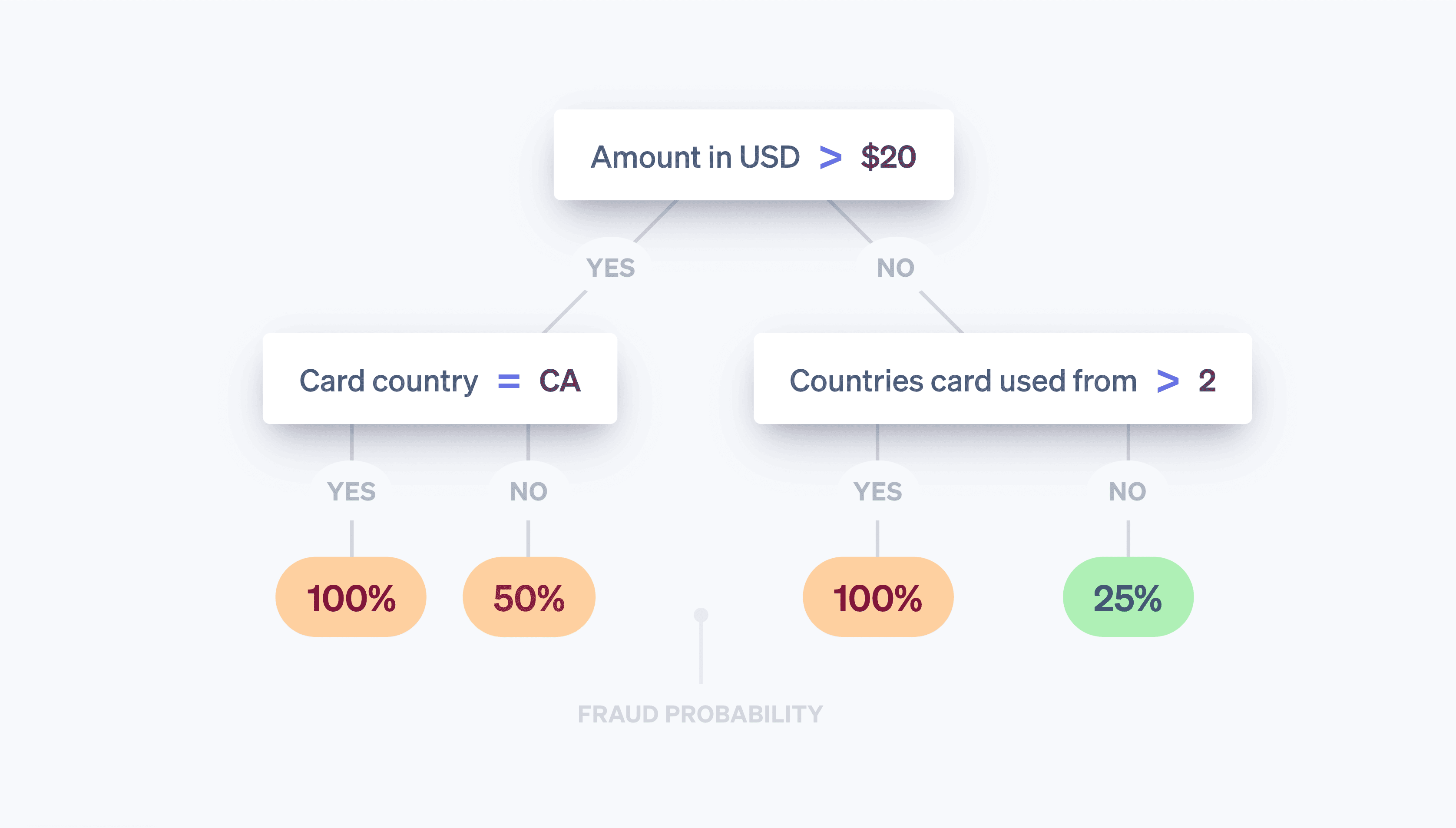
When we observe a new transaction, we look at the input values and traverse the tree “20-questions style” until we reach one of its “leaves.” Each leaf consists of all the samples in the data set (the table above) satisfying the question-answer pairs along the path we followed down the tree, and the probability that we think the new transaction is fraudulent is the number of samples in the leaf that are fraudulent divided by the total number of samples in the leaf. Put another way, the tree answers the question, “Of transactions in our data set with properties similar to the transaction we’re examining now, what fraction was actually fraudulent?” The machine learning part is concerned with the construction of the tree—what questions do we ask, in what order, to maximize the chances that we can distinguish between the two classes accurately? Decision trees are particularly easy to visualize and reason about, but there are many different learning algorithms, each with their own unique way of representing the relationships we are trying to model.
Today’s machine learning models are prevalent—powering, behind the scenes, many of the products we frequently interact with—and generally much more sophisticated than the toy model above:
- Google accurately and precisely provides spelling suggestions with its “Did you mean?” feature in Search using machine learning to model millions of language-related parameters in less than three seconds.
- Amazon uses machine learning to predict purchases with its recommendation system based on the needs, preferences, and changing behaviors of users across its entire platform, even for new users with no historical data.
And, most relevant to this discussion, machine learning is the basis for Stripe Radar, which seeks to predict which of your payments are fraudulent.
How does machine learning work?
Academic machine learning courses will usually focus on the modeling process—the methods for translating data (e.g., the table above) into the models (e.g., the decision tree), which are the algorithms that tell you how input values (the country in which the card was issued, the number of countries where the card was used, etc.) map to output values (was the transaction fraudulent or not?). The process that takes the input data table above and produces the “best” tree is an example of a particular machine learning method. Modeling involves a number of steps, which depend on the nature of your data and the models you chose to use. While we won’t go into too much detail, a high-level overview follows.
First, we need to obtain training data. Before we can begin automatically detecting fraud, we need a dataset with examples of it. For each example, we need to have recorded (or be able to compute retrospectively) a range of input properties that could be useful in making future predictions about the output value. These input properties are called features. The collection of inputs together for a given sample is a feature vector. In our example above, the feature vector had a length of three (the country in which the card was issued, the number of countries where the card was used in the past day, and the payment amount in USD).
However, feature vectors with hundreds or thousands of features are not uncommon. In fact, Radar uses hundreds of features and most of them are aggregates computed from across the Stripe network. As our network size expands, each feature becomes more informative because our training data becomes more representative of the feature’s entire data set, including all non-Stripe data. The output value—in our running example, the boolean as to whether or not the transaction was fraudulent—is often called a target or label. The training data thus consists of a large number of feature vectors and their corresponding output values.
Second, we need to train a model. Given the training data, we need a method for producing our predictive model. Machine learning classifiers generally do not just output a class label—they typically assign probabilities that the given sample belongs to each possible class. For example, the output of a fraud classifier might be an assessment that the payment has a 65% chance of being fraudulent and a 35% chance of being legitimate.
There are many machine learning techniques that can be used to train models. For most industrial machine learning applications, traditional approaches like linear regression, decision trees, or random forests do just fine.
However, sophisticated techniques, namely neural nets and deep learning, inspired by the architecture of neurons in the brain, are responsible for many advances in the field, including AlphaFold’s predictions for 98% of all human proteins. The real advantages of neural nets only come when they’re trained on very large datasets, so in practice, many businesses aren’t able to take full advantage of them. Because of the size of our network, Stripe is able to take this more cutting-edge approach to deliver real results to our users. Our new models have improved Radar’s machine learning performance by over 20% year over year, helping us detect more fraud while keeping false positives low.
Feature engineering
One of the most involved parts of industrial machine learning is feature engineering. Feature engineering consists of two parts:
(1) formulation of features that have predictive value based on extensive knowledge of the problem domain and (2) engineering to make the values of those features available both for model training and for model evaluation in “production.”
In formulating a feature, a Stripe data scientist may have a hunch that a useful feature would be to compute whether the card payment is coming from an IP address that is common for that card. For example, a card payment originating from IP addresses seen before (like the home or workplace of the cardholder) is less likely to be fraudulent than if the IP address was from a different state. In this case, the idea is intuitive, but generally these hunches come from examining thousands of cases of fraud. For example, you may be surprised to learn that computing the difference between the time on the user device and the current Coordinated Universal Time (UTC) or the count of countries in which the card was successfully authorized helps detect fraud.
Once we have the feature idea, we need to compute its historical values so that we can train a new model including the feature—this is the process of adding a new column to the “table” of data we use to produce our model. To do this for our candidate feature, for every payment in Stripe’s history, we need to compute the two most frequent IP addresses from which preceding payments were made with the card. We might do this in a distributed fashion with a Hadoop job, but even then we may find that the job takes too much time (or memory). We might then try optimizing the computation by using a space-saving probabilistic data structure. Even for features that are intuitively simple, producing data for model training requires dedicated infrastructure and established workflows.
Not all features are handcrafted by engineers; some can be left for the model to compute with subsequent testing before deployment. Categorical values, such as the country of origin of a card or the merchant that processed a transaction (as opposed to numerical features), lend themselves well to this approach. These features often have a wide range of values, and defining a good representation for them can be challenging.
At Stripe, we train our models to learn an embedding for each merchant based on transaction patterns. An embedding can be thought of as the coordinates of the individual merchant compared to others. Similar merchants will often have similar embeddings (as measured by cosine distance), allowing the model to transfer learnings from one merchant to the next. The table below shows how these embeddings could look, given that Uber and Lyft are likely more similar to each other than to Slack. At Stripe, we use embeddings for a variety of categorical features, such as issuing bank, merchant and user country, day of the week, and more.
|
Illustrative embedding coordinates
|
|||
|---|---|---|---|
|
Uber
|
2.34 | 1.1 | -3.5 |
|
Lyft
|
2.1 | 1.2 | -2 |
|
Slack
|
7 | -2 | 1 |
The use of embeddings is increasingly common in large-scale industrial applications of machine learning. Word embeddings like these, for example, help capture the complex semantic relationships between words and have been involved in natural language processing milestones like Word2Vec, BERT, and GPT-3. Stripe produces embeddings to capture similarity relationships between different entities on the Stripe network the same way that the methods above capture similarities between words. Embeddings are a powerful way to learn higher-level concepts without explicit training. For example, fraud patterns are often unevenly distributed geographically. With embeddings, if our system identifies a new fraud pattern in Brazil, it can automatically identify the same pattern if it appears in the US, without further training. In this way, algorithmic advances help stay ahead of shifting fraud patterns, protecting our customers.
If you are interested in working on machine learning products at Stripe, get in touch!
Evaluating machine learning models
Once we’ve developed a machine learning classifier for fraud that uses hundreds of features and assigns a probability (or score) that the payment is fraud to every incoming transaction, we need to determine how effective the model is at detecting fraud.
Key terms
To better understand how we evaluate our machine learning systems, it’s useful to define some key terms.
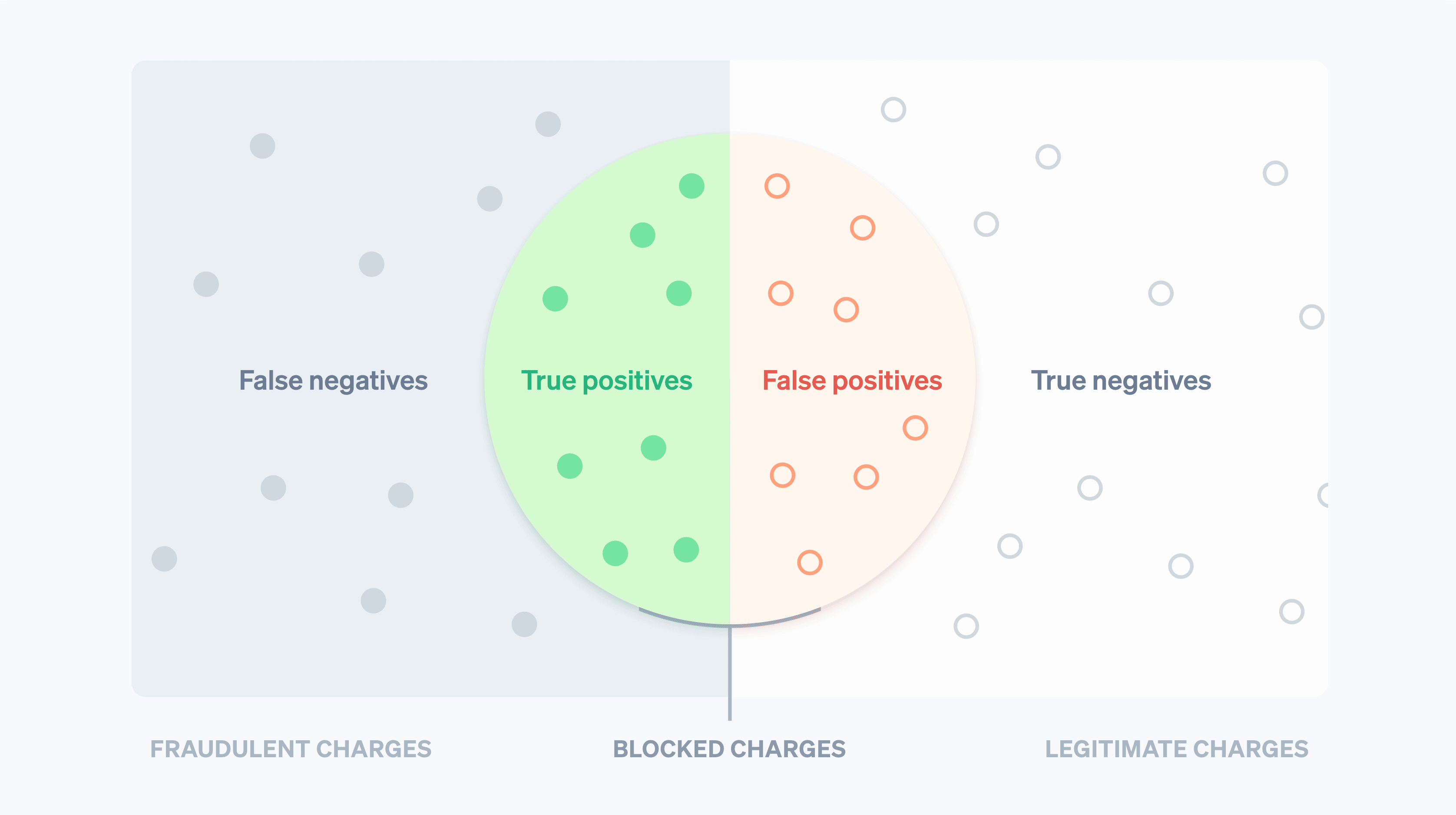
Let’s start by supposing we’ve created a policy to block a payment if the machine learning model assigns the transaction a probability of being fraudulent of at least 0.7. (We write this as P(fraud)>0.7). Here are some quantities useful for reasoning about the performance of our model and policy:
Precision: The precision of our policy is the fraction of transactions we block that are actually fraudulent. The higher the precision is, the fewer false positives there are. Let’s say out of 10 transactions, P(fraud)>0.7 for six and, of those six, four are actually fraudulent. The precision is then 4/6=0.66.
Recall: Also known as sensitivity or the true positive rate, recall is the fraction of all fraud that is caught by our policy; that is, the fraction of fraud for which P(fraud)>0.7. The higher the recall is, the fewer false negatives there are. Let’s say out of 10 transactions, five are actually fraudulent. If four of these transactions are assigned a P(fraud)>0.7 by our model, then recall is 4/5=0.8.
False positive rate: The false positive rate is the fraction of all legitimate payments that are incorrectly blocked by our policy. Let’s say out of 10 transactions, five are legitimate. If two of these transactions are assigned a P(fraud)>0.7 by our model, then the false positive rate is 2/5=0.4.
While there are other quantities that are used when evaluating a classifier, we’ll focus on these three.
Precision-recall and ROC curves
The next natural question is what good values are for the precision, recall, and false positive rate. In a theoretically ideal world, precision would be 1.0 (that is, 100% of transactions that you classify as fraud are actually fraud), which would make your false positive rate 0 (you didn’t incorrectly classify a single legitimate transaction as fraudulent), and recall would also be 1.0 (100% of fraud is identified as such).
In reality, there is a tradeoff between precision and recall—as you increase the probability threshold for blocking, precision will increase (since the criterion for blocking is more stringent) and recall will decrease (since fewer transactions match the high probability criterion). For a given model, a precision-recall curve captures the tradeoff between precision and recall as the policy threshold is varied:
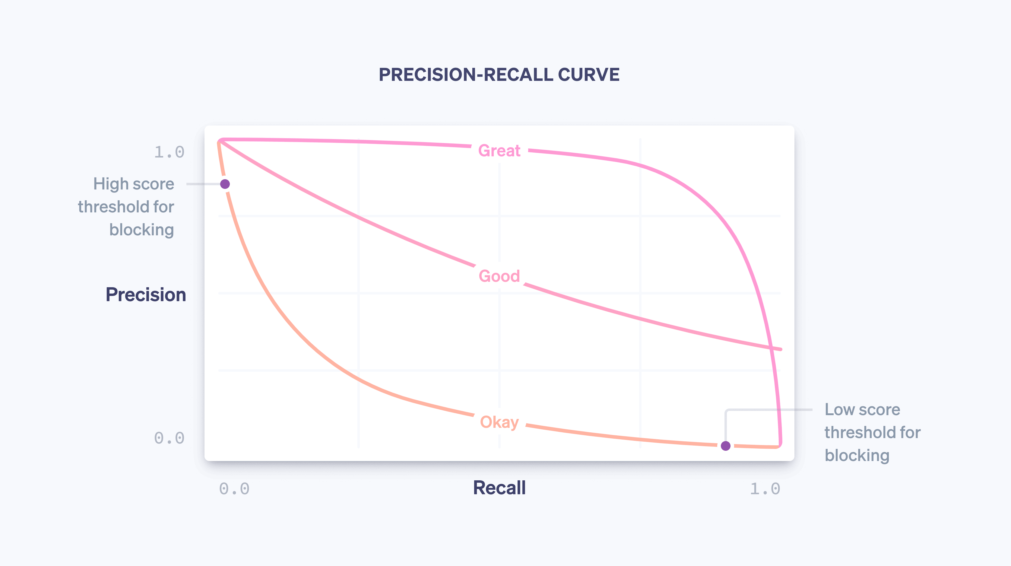
As our model gets better overall—due to training more and more data from across the Stripe network, adding features that are good predictors of fraud, and tweaking other model parameters—the precision-recall curve will change, as depicted in the example above. As it controls the trade-off for businesses on Stripe, we closely monitor the impact on the precision-recall curve when our data scientists and machine learning engineers modify models.
When considering a precision-recall graph, it’s important to distinguish between the two notions of “performance.” On its own, a model is better overall the closer it hugs the top-right of the chart (that is, where precision and recall are both 1.0). However, operationalizing a model usually requires the selection of an operating point on the precision-recall curve (in our case, the policy threshold for blocking a transaction), which controls the concrete impact using the model has on a business.
Put simply, there are two problems:
The data science problem of producing a good machine learning model by adding the right features. The model controls the shape of the precision-recall curve.
The business problem of picking a policy to decide how much potential fraud to block. The policy controls where on the curve we’re operating.
Another curve that is examined when evaluating a machine learning model is the ROC curve. (ROC is short for “receiver operating characteristic,” a relic of the curve’s origin in signal processing applications.) The ROC curve is a plot of the false positive rate (on the x-axis) and the true positive rate (which is the same as the recall) on the y-axis for various values of the policy threshold.
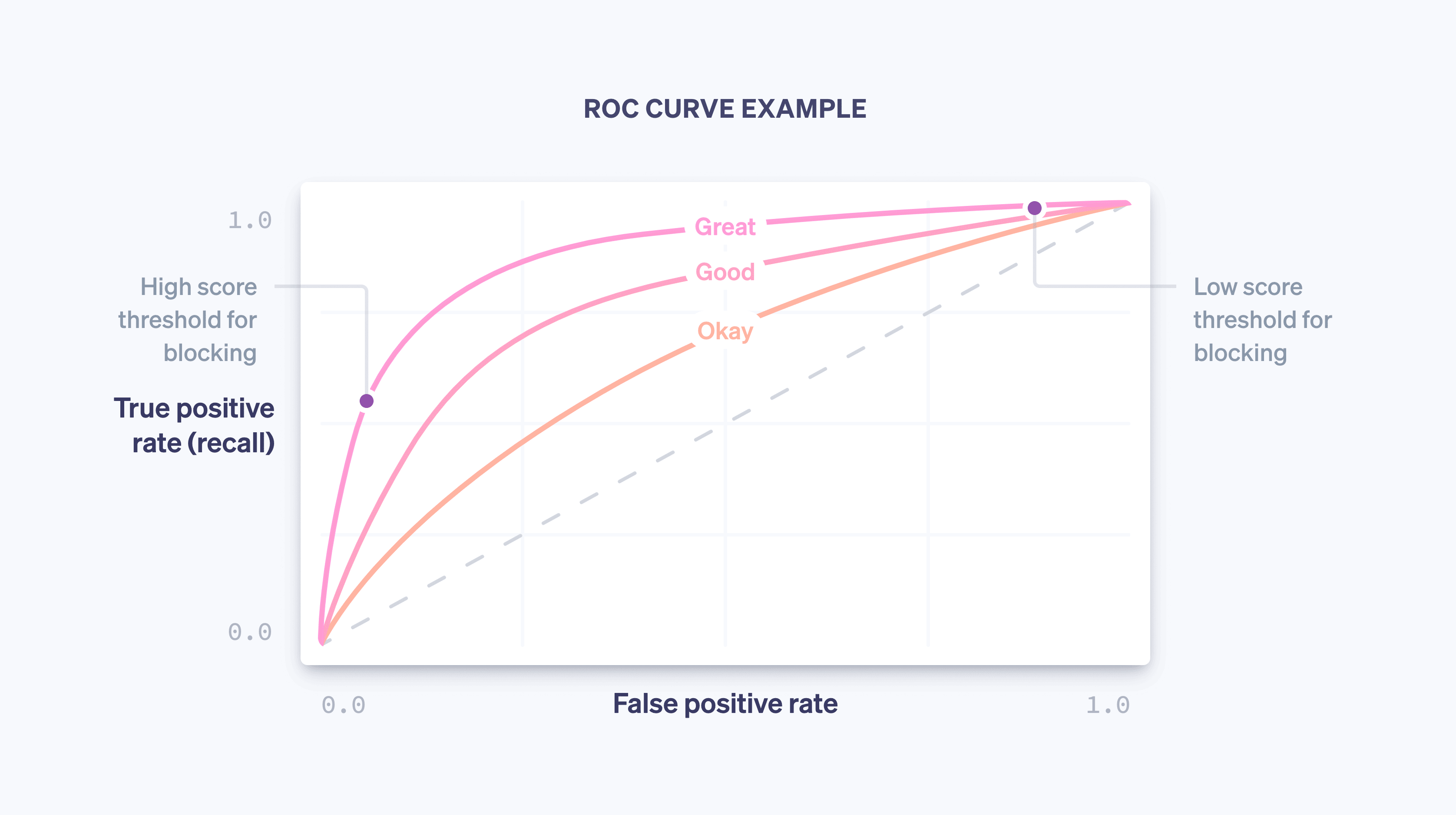
The ideal ROC will hug the top left of the graph (where recall is 1.0 and the false positive rate is 0.0), and as the model improves, the ROC will move more in that direction. One way to capture the overall quality of the model is by computing the area under the curve (or AUC); in the ideal case, the AUC will be 1.0. When developing our models, we look to see how the precision-recall curve, the ROC curve, and the AUC change.
Score distributions
Imagine that we have a model that randomly assigns a probability of fraud between 0.0 and 1.0 to a transaction. Practically, this model does nothing to discriminate between legitimate and fraudulent transactions and is of little use to us. This randomness is captured by the score distribution of the model—the fraction of transactions getting each possible score. In the completely random case, the score distribution would be close to uniform:
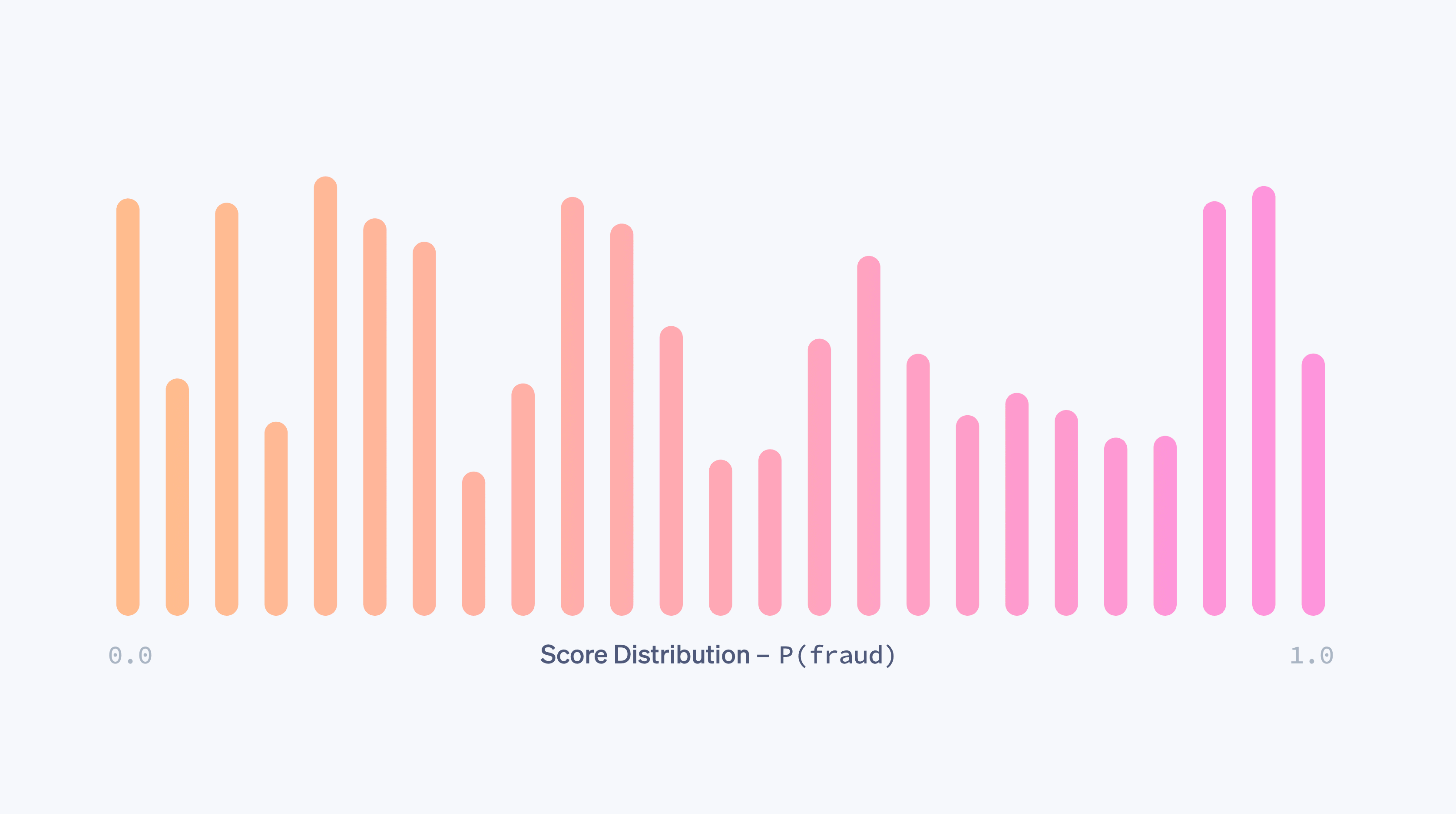
A model will have a uniform score distribution like the above if, for example, the model has no features that are even remotely predictive of fraud. As a model is improved—by adding predictive features, training on more data, and so forth—its power to discriminate between the fraudulent and legitimate classes will increase and the score distribution will become more bimodal, with peaks around the scores of 0.0 and 1.0.
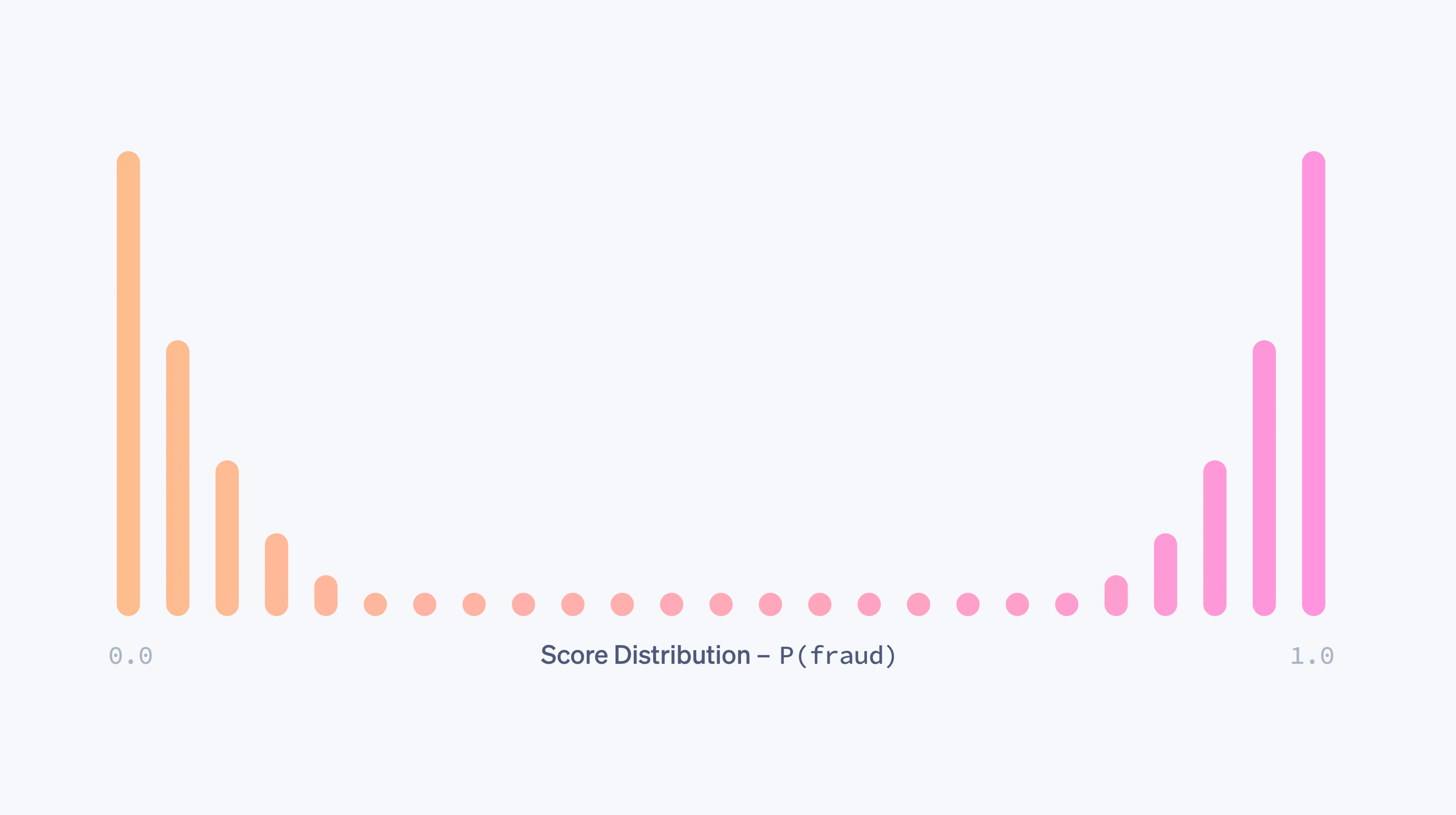
On its own, a bimodal distribution does not tell you that a model is good. (A vacuous model that randomly assigns probabilities of just 0.0 and 1.0 would also have a bimodal score distribution.) However, in the presence of evidence that transactions with a low score are not fraudulent and transactions with a high score are fraudulent, an increasingly bimodal distribution is a sign of improved efficacy for a model.
Different models will often have different score distributions. When we release new models, we compare the old and updated distributions, in order to minimize any disruptive changes caused by a sudden shift in scores. In particular, we take into account merchants’ current block policies as measured by the threshold at which they block transactions, and aim to keep the proportion of transactions that falls above the threshold stable.
Computing precision and recall
We can compute the metrics above in two different contexts: during model training, using the historical data that drives the model development process, and after model deployment, using production data; that is, data from the world when the model is already being used to take action by, say, blocking transactions if P(fraud)>0.7.
For the former, data scientists will typically take the training data they have (reference the table from above) and randomly assign some fraction of the records to a training set and the other records to a validation set. One could imagine that the first 80% of rows go into the former and the last 20% into the latter, for example.
The training set is the data fed into a machine learning method to produce a model as described above. Once we have a candidate model, we can then use it to assign scores to each sample in the validation set. The validation set scores together with their output values are used to compute the ROC and precision-recall curves, the score distributions, and so forth. The reason we use a separate validation set that is held out from the training set is that the model has already “seen the answer” for its training examples and learned from these answers. A validation set helps us generate metrics that are an accurate measure of the predictive power of the model on new data.
Machine learning operations: deploying models safely and frequently
Once a model’s performance has been shown to outperform the current production model on a held out set, the next step is to deploy it to production. There are two key challenges to this process:
Real-time computations: We need to be able to compute the value of every feature for every new payment in real time because we want to be able to block all transactions that our classifier believes are likely to be fraudulent. This computation is entirely separate from the one used to produce training data—we need to maintain an up-to-date state on the two most frequently used IP addresses for every card ever seen at Stripe, and fetching and updating those counts needs to be fast because those operations happen as part of the Stripe API flow. Machine learning infrastructure teams at Stripe have made this easier by building systems to specify features in a declarative way and making the current values of the features available automatically in production with low latency.
Real-world user application: Deploying a machine learning model is different from deploying code. While code changes are often validated with precise test cases, model changes are usually tested on a large aggregate dataset using metrics such as the ones we defined above. But a model that is better at catching fraud in aggregate may not be better for every Stripe user. It may be that the improvement in performance is unevenly distributed, with a few large merchants seeing large gains while many small merchants see small regressions. A model may have higher recall but cause a spike in block rate, which would be disruptive to businesses (and their customers). Before we release a model, we verify that it performs well in practice. To do so, we measure the change each model would cause to a variety of metrics, such as false positive rate, block rate, and authorization rate on an aggregated and per merchant basis for a subset of Stripe users. If we find that a new model would cause an undesirable shift in one of those guardrail metrics, we adjust it for different subsets of users before releasing it to minimize disruptions and ensure optimal performance.
We’ve found that automating as much of the training and evaluation process as possible provides compounding benefits to model iteration speed. In the last year, we’ve invested in tooling to automatically and regularly train, tune, and evaluate models using our latest features and model architecture. For example, we continuously update performance dashboards after a model is trained—before it is released. That way, an engineer can easily detect if a model candidate has gotten stale on a subset of traffic before even releasing it and proactively retrain it.
After we release a model, we monitor its performance and start working on the next release. Because fraud trends change quickly, machine learning models quickly start experiencing drift: The data they were trained on no longer is representative of fraud today.
Using these tools, we’ve tripled the speed at which we release models, translating directly to large performance gains in production. In fact, even retraining a model from last month on more recent data (using the same feature definitions and architecture) and releasing it allows us to increase our recall by as much as half a percentage point each month. Being able to release models frequently and safely allows us to capitalize on and compound the gains of feature engineering and modeling work and adapt to changing fraud patterns for Radar users.
Once we put a model into production, we continuously monitor the performance of our model-policy pair. For payments that have scores below the threshold for blocking, we can observe the ultimate outcome—was the transaction disputed by the cardholder as fraud? Payments that have scores above the threshold, however, are blocked, and so we can’t know what their outcomes would have been. Computing the full production precision-recall or ROC curve is thus more involved than computing the validation curves because it involves counterfactual analysis—we need to obtain statistically sound estimates of what would have happened even to the payments we blocked. Over the years, Stripe has developed methods to do this, which you can learn more about in this talk.
We’ve just described a few of the measures of model efficacy that data scientists and machine learning engineers look at when developing machine learning models. Next, we’ll talk about how businesses should think about fraud prevention.
How Stripe can help
Fixating on just one number to capture your fraud performance may result in choices that are not optimal for your business. We’ve found that businesses will often overemphasize false negatives—they’re very concerned about fraud that is missed—and underemphasize false positives. This mindset often results in ineffective and costly brute-force measures like blocking all international cards. In general, you should be thinking about how all the various performance measures relate and what the right trade-offs are given your particular circumstances. Here’s an example of how these metrics tie together to help you determine the efficacy of your fraud prevention system:
APPROXIMATE MODEL FOR BREAK-EVEN PRECISION
If your average sale is $26 with a margin of 8%, your profit per sale is $26.00 × 8.00% = $2.08. On average, if your product costs $26.00 – $2.08 = $23.92 to produce and you’re levied a chargeback fee of $15, your total loss for a fraudulent sale is $23.92 + $15.00 = $38.92. Therefore, one fraudulent sale costs you the profit of $38.92 / $2.08 = 18.71 legitimate sales, and your break-even precision is 1 / (1 + 18.71) = 5.07%.
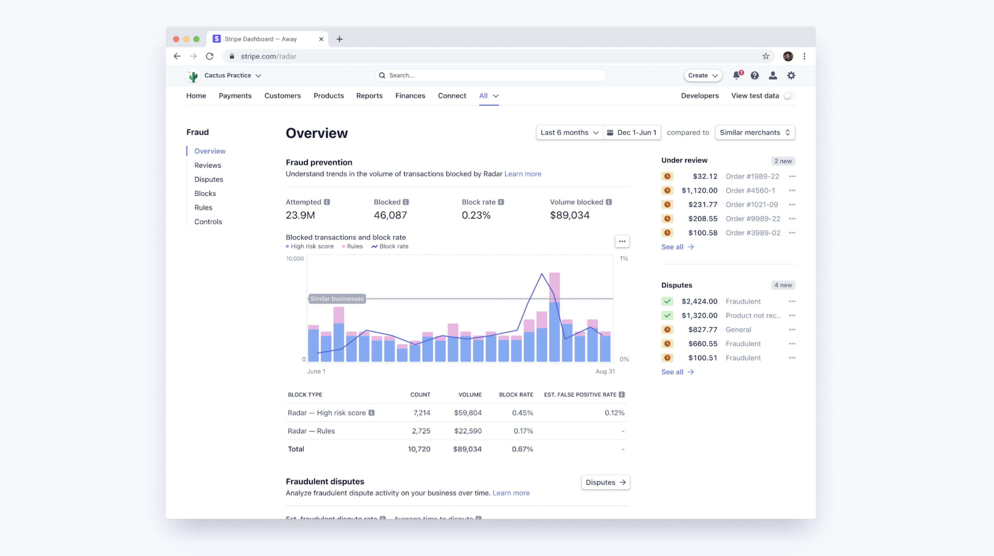
Radar’s machine learning thresholds trade off optimizing for merchants’ margins and keeping block rates stable across our user base. You can access a dashboard to see how Radar’s machine learning is performing for your business, as well as your custom rules performance if you’re using Radar for Fraud Teams. These tools enable you to easily compare your fraudulent dispute rates, false positive rates, and block rates to other similar businesses based on aggregated, custom cohorts of businesses that are in similar verticals or sizes to yours.
Improving performance with rules and manual reviews
With Radar for Fraud Teams, you can fine tune your protection by directly adjusting your risk threshold to block or allow more payments. Alongside the more automatic machine learning algorithms, Radar for Fraud Teams also lets individual businesses compose customized rules (for example, “block all transactions above $1,000 when the IP country does not match the card’s country”), request interventions, and manually review flagged payments in the Dashboard.
Such rules can be seen as simple “models” (they can be represented as decision trees, after all!), and they should be evaluated—with a full consideration of the tradeoff between precision and recall—in the same way as models. When you create a rule with Radar, we’ll present historical statistics on the number of matching transactions that were actually disputed, refunded, or accepted to help aid with these calculations before the rule is even implemented. Once live, you can see the impact on false positive and dispute rates by rule.
Just as important, rules, interventions, and manual reviews allow users to change the shape of the precision-recall curve in their favor by adding in proprietary, business-specific logic (rules) or by expending some additional effort (manual review).
If you realize that the machine learning algorithms are frequently missing a certain type of fraud particular to your business (and that fraud is easily identifiable to you), you can compose a rule to block it. That specific intervention will typically increase recall with little cost to precision, in effect moving the operating point along a less steep, more favorable precision-recall curve.
By sending some classes of transactions to manual review instead of blocking them outright, you can gain precision without a hit to recall. Similarly, by sending some transactions to manual review instead of allowing them outright, you can gain recall without a hit to precision.
Of course, in these cases, you are paying for these gains with additional human work (and exposing yourself to the accuracy of your team’s assessments), but having manual review, rules, and interventions to authenticate high-risk customers as additional tools gives you another lever to optimize fraud outcomes.
Next steps
We hope this guide helps you understand how machine learning is applied to fraud prevention at Stripe and how to gauge the efficacy of your fraud systems. You can learn more about Radar’s features or explore our docs.
If you have any questions or would like to learn more about Stripe Radar, please reach out.